Joint Clustering Analysis

suppressPackageStartupMessages({
    library(ggplot2)
    library(patchwork)
    library(scater)
    library(harmony)
    library(BayesSpace)
})
set.seed(100)

In this vignette, we describe how to perform a joint clustering analysis of 4 serial sections of the dorsolateral prefrontal cortex. The samples are 151673-151676, first described by Maynard et al. (2021).

Loading and preprocessing data

The samples are available in the BayesSpace package via the getRDS() function. The plots of the ground truth clusters (which were obtained through manual expert annotation) suggest that jointly modeling the samples may be beneficial.

sce1 = getRDS("2020_maynard_prefrontal-cortex", "151673")
sce2 = getRDS("2020_maynard_prefrontal-cortex", "151674")
sce3 = getRDS("2020_maynard_prefrontal-cortex", "151675")
sce4 = getRDS("2020_maynard_prefrontal-cortex", "151676")

((clusterPlot(sce1, "layer_guess_reordered", color = NA) |
  clusterPlot(sce2, "layer_guess_reordered", color = NA)) /
  (clusterPlot(sce3, "layer_guess_reordered", color = NA) |
  clusterPlot(sce4, "layer_guess_reordered", color = NA))) +
  plot_layout(guides = "collect") +
  plot_annotation(title = "Ground truth")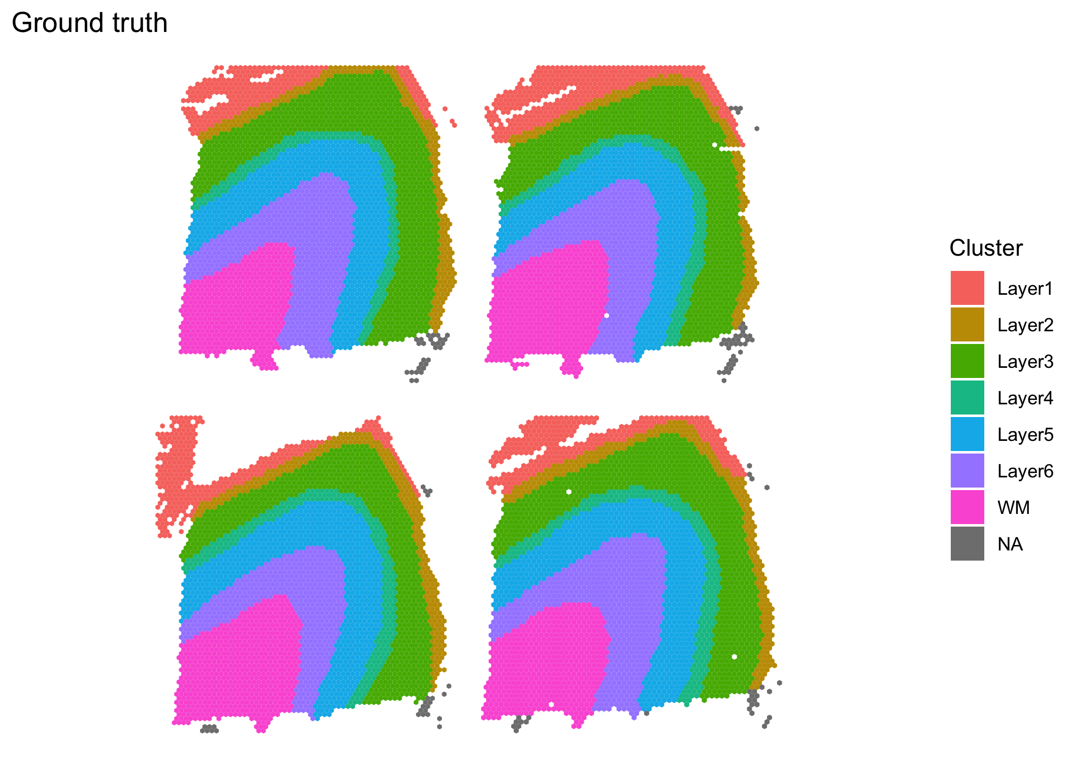

The rowData for each sample contains previously calculated highly variable genes (HVGs), which are not consistent across samples. These need to be removed and recalculated after combining into one SingleCellExperiment object.

rowData(sce1)$is.HVG = NULL 
rowData(sce2)$is.HVG = NULL 
rowData(sce3)$is.HVG = NULL 
rowData(sce4)$is.HVG = NULL 

#Combine into 1 SCE and preprocess
sce.combined = cbind(sce1, sce2, sce3, sce4, deparse.level = 1)
sce.combined = spatialPreprocess(sce.combined, n.PCs = 50) #lognormalize, PCA

Batch correction

We aim for our clustering analysis to capture biological patterns across the four samples rather than technical differences between each sample. It is a good idea to check for batch effects first by plotting a low-dimensional representation of the data. Note here the sample name is stored in colData(sce.combined) in the column sample_name.

sce.combined = runUMAP(sce.combined, dimred = "PCA")
colnames(reducedDim(sce.combined, "UMAP")) = c("UMAP1", "UMAP2")

ggplot(data.frame(reducedDim(sce.combined, "UMAP")), 
       aes(x = UMAP1, y = UMAP2, color = factor(sce.combined$sample_name))) +
  geom_point() +
  labs(color = "Sample") +
  theme_bw()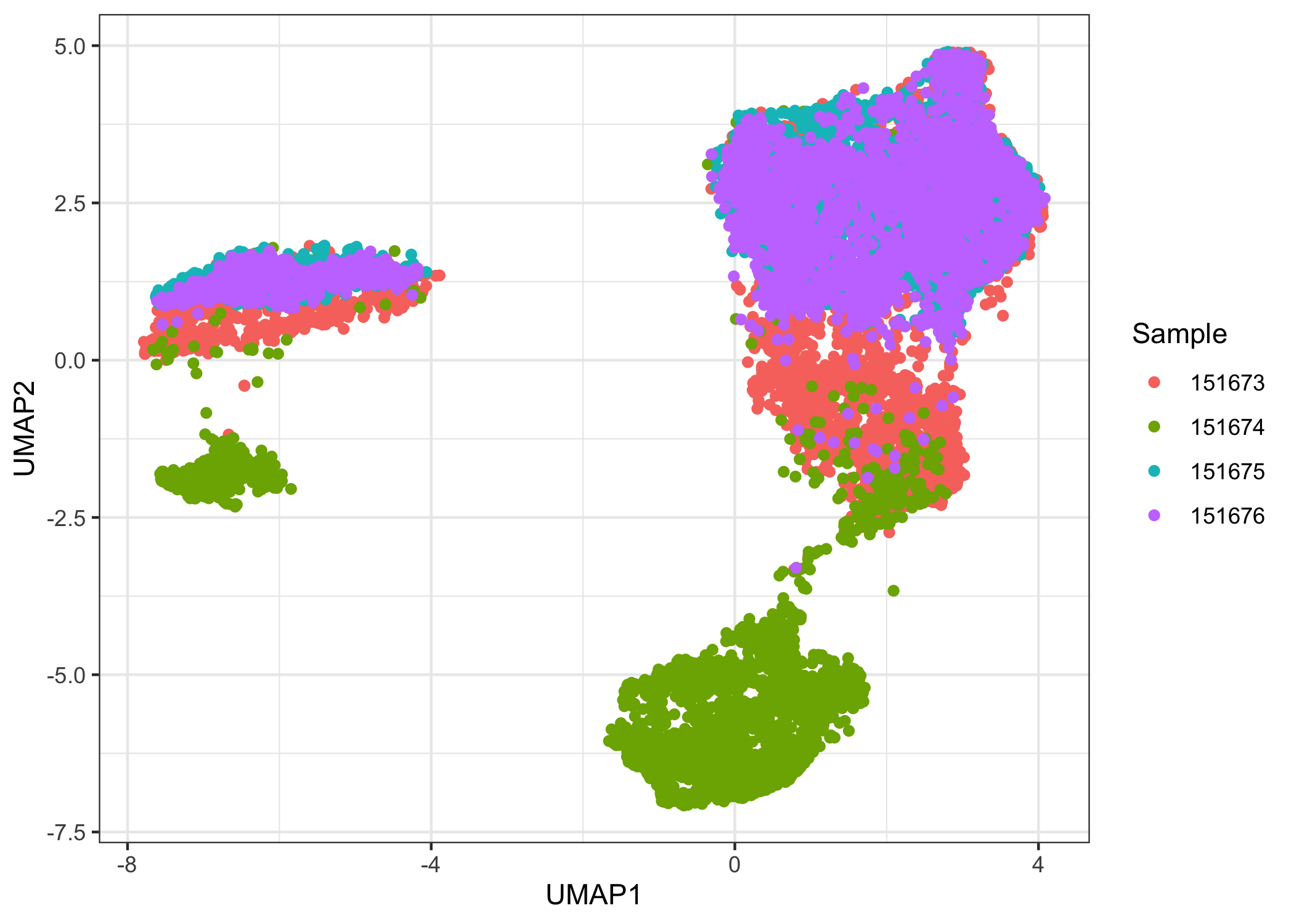

plot of chunk batch

There is a noticeable batch effect. We use Harmony to integrate the four samples.

# install.packages("devtools")
# devtools::install_github("immunogenomics/harmony")

sce.combined = RunHarmony(sce.combined, "sample_name", verbose = F)
sce.combined = runUMAP(sce.combined, dimred = "HARMONY", name = "UMAP.HARMONY")
colnames(reducedDim(sce.combined, "UMAP.HARMONY")) = c("UMAP1", "UMAP2")

ggplot(data.frame(reducedDim(sce.combined, "UMAP.HARMONY")), 
       aes(x = UMAP1, y = UMAP2, color = factor(sce.combined$sample_name))) +
  geom_point() +
  labs(color = "Sample") +
  theme_bw()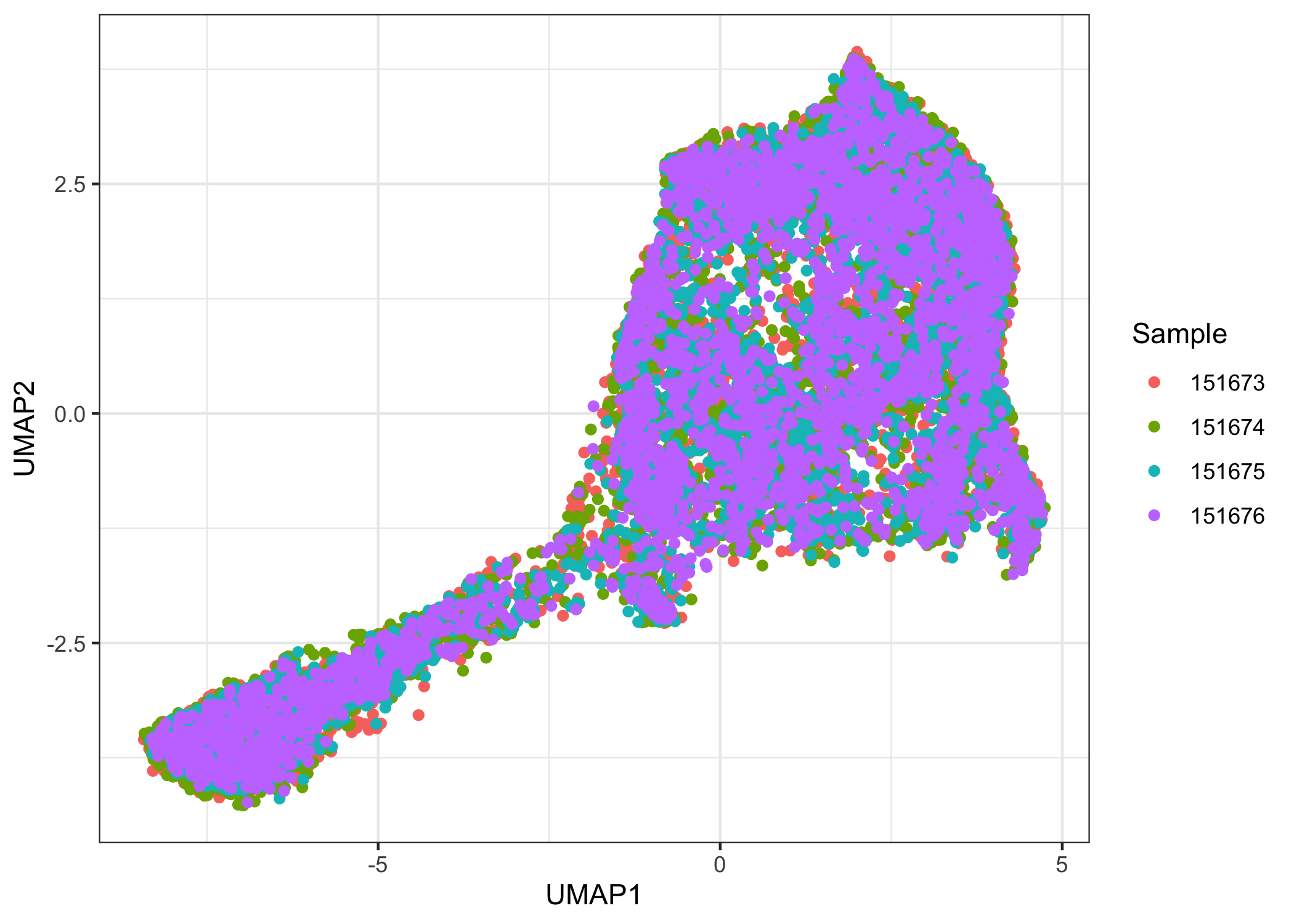

plot of chunk harmony

Clustering

After integration, there appears to be no obvious batch effect. We now prepare the samples for joint clustering. The spatial locations for each sample need to be offset so that spots of different samples are not neighbors. Here, we add 100 to row and/or 150 to col to achieve this effect. In this dataset, row ranges from 0 to 77 while col ranges from 0 to 127. Here, row and col are also columns of colData(sce.combined).

sce.combined$row[sce.combined$sample_name == "151674"] = 
  100 + sce.combined$row[sce.combined$sample_name == "151674"]
sce.combined$col[sce.combined$sample_name == "151675"] = 
  150 + sce.combined$col[sce.combined$sample_name == "151675"]
sce.combined$row[sce.combined$sample_name == "151676"] = 
  100 + sce.combined$row[sce.combined$sample_name == "151676"]
sce.combined$col[sce.combined$sample_name == "151676"] = 
  150 + sce.combined$col[sce.combined$sample_name == "151676"]
clusterPlot(sce.combined, "sample_name", color = NA) + #make sure no overlap between samples
  labs(fill = "Sample", title = "Offset check")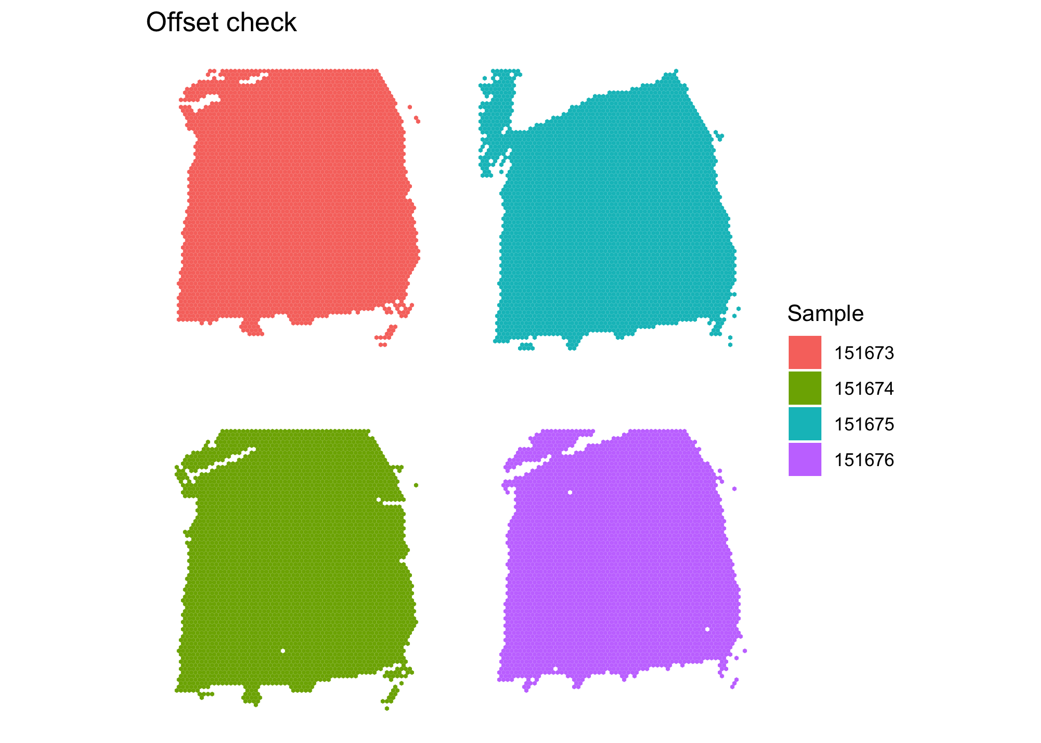

plot of chunk offset

The plot shows the samples are not overlapping, so the neighborhood network will be detected correctly. We proceed to use BayesSpace for clustering.

sce.combined = spatialCluster(sce.combined, use.dimred = "HARMONY", q = 7, nrep = 10000) #use HARMONY
clusterPlot(sce.combined, color = NA) + #plot clusters
  labs(title = "BayesSpace joint clustering")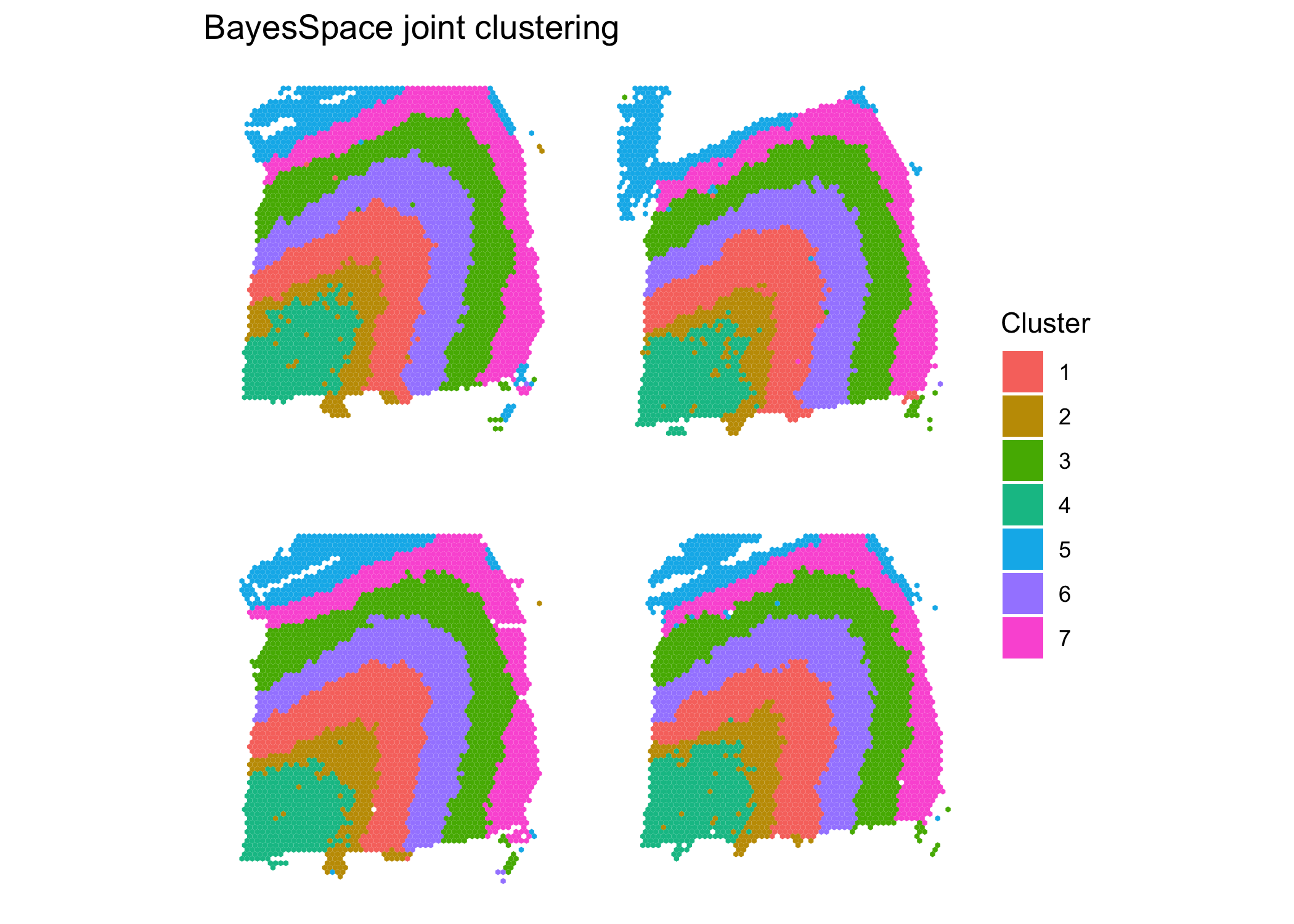

plot of chunk cluster

#calculate ARIs
aris = rep(NA, 4)
names(aris) = 151673:151676
for (sample.id in 151673:151676){
  aris[as.character(sample.id)] = 
    mclust::adjustedRandIndex(sce.combined$spatial.cluster[sce.combined$sample_name == sample.id],
                              sce.combined$layer_guess[sce.combined$sample_name == sample.id]) 
}

The results of the joint clustering show consistent structure across samples. Comparing to the ground truth, we obtain ARIs of 0.56, 0.59, 0.6, and 0.57 for the four samples. This represents a substantial improvement over the single sample clustering analyses, where we obtained values of 0.55, 0.44, 0.55, and 0.37 respectively for the four samples.

Edward Zhao, Matt Stone, and Raphael Gottardo

2021-08-03

Loading and preprocessing data

Batch correction

Clustering